In Feature-Distributed Clustering (FDC), we show how cluster ensembles can be used to boost quality of results by combining a set of clusterings obtained from partial views of the data. As mentioned in the introduction, such scenarios result in distributed databases and federated systems that cannot be pooled into one big flat file because of proprietary data aspects, privacy concerns, performance issues, etc. In such situations, it is more realistic to have one clusterer for each database and transmit only the cluster labels (but not the attributes of each record) to a central location where they can be combined using the supra-consensus function.
For our experiments, we simulate such a scenario by running several clusterers, each having access to only a restricted, small subset of features (subspace). Each clusterer has a partial view of the data. Each clusterer has access to all objects. The clusterers find groups in their views/subspaces using the same clustering technique. In the combining stage, individual results are integrated using our supra-consensus function to recover the full structure of the data. As this is a knowledge-reuse framework, the ensemble has no access to the original features.
|
|
First, let us discuss experimental results for the 8D5K data,
since they lend themselves well to illustration.
We create 5 random 2D views (through selection of a pair of features)
of the 8D data, and use Euclidean-based graph partitioning with ![]() in each view to obtain 5 individual clusterings. The 5 individual
clusterings are then combined using our supra-consensus function proposed in
the previous section.
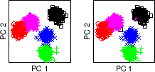
The clusters are linearly separable in the full 8D space and
clustering in the 8D space yields the original generative labels and
is referred to as the reference clustering. Using PCA to project the
data into 2D separates all 5 clusters fairly well (figure
5.10). In figure 5.10(a), the
reference clustering is illustrated by coloring the data points in the
space spanned by the first and second principal components (PCs).
Figure 5.10(b) shows the final FDC result after
combining 5 subspace clusterings. Each clustering has been computed
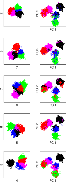
from random feature pairs. These subspaces are shown in figure
5.9. Each of the rows corresponds to a random
selection of 2 out of 8 feature dimensions. For each of the 5 chosen
feature pairs, a row shows the 2D clustering (left, feature pair shown
on axis) and the same 2D clustering labels used on the data projected
onto the global 2 principal components (right).
For consistent appearance of clusters across rows, the dot
colors / shapes have been matched using meta-clusters. All points in
clusters of the same meta-cluster share the same color / shape amongst
all plots.
In any subspace, the clusters can not be segregated well due to strong
overlaps. The supra-consensus function can combine the partial knowledge of
the 5 clusterings into a far superior clustering.
FDC (figure 5.10(b)) are
clearly superior compared to any of the 5 individual results (figure
5.9(right)) and is almost flawless compared to
the reference clustering (figure 5.10(a)). The best
individual result has 120 `mislabeled' points while the consensus only
has 3 points `mislabeled'.
in each view to obtain 5 individual clusterings. The 5 individual
clusterings are then combined using our supra-consensus function proposed in
the previous section.
The clusters are linearly separable in the full 8D space and
clustering in the 8D space yields the original generative labels and
is referred to as the reference clustering. Using PCA to project the
data into 2D separates all 5 clusters fairly well (figure
5.10). In figure 5.10(a), the
reference clustering is illustrated by coloring the data points in the
space spanned by the first and second principal components (PCs).
Figure 5.10(b) shows the final FDC result after
combining 5 subspace clusterings. Each clustering has been computed
from random feature pairs. These subspaces are shown in figure
5.9. Each of the rows corresponds to a random
selection of 2 out of 8 feature dimensions. For each of the 5 chosen
feature pairs, a row shows the 2D clustering (left, feature pair shown
on axis) and the same 2D clustering labels used on the data projected
onto the global 2 principal components (right).
For consistent appearance of clusters across rows, the dot
colors / shapes have been matched using meta-clusters. All points in
clusters of the same meta-cluster share the same color / shape amongst
all plots.
In any subspace, the clusters can not be segregated well due to strong
overlaps. The supra-consensus function can combine the partial knowledge of
the 5 clusterings into a far superior clustering.
FDC (figure 5.10(b)) are
clearly superior compared to any of the 5 individual results (figure
5.9(right)) and is almost flawless compared to
the reference clustering (figure 5.10(a)). The best
individual result has 120 `mislabeled' points while the consensus only
has 3 points `mislabeled'.
We also conducted FDC experiments on the other three data-sets. Table
5.3 summarizes the results and several comparison benchmarks.
The choice of the number of random subspaces ![]() and their
dimensionality is currently driven by the user.
For example, in the YAHOO case, 20 clusterings were performed in
128-dimensions (occurrence frequencies of 128 random words) each. The
average quality amongst the results was 0.17 and the best quality was
0.21. Using the supra-consensus function to combine all 20 labelings yields
a quality of 0.38, or 124% higher mutual information than the
average individual clustering.
In all scenarios, the consensus clustering is as good or better than
the best individual input clustering and always better than the
average quality of individual clusterings.
When processing on the all features is not possible and only
limited views exist, a cluster ensemble can boost results
significantly compared to individual clusterings.
Also,
since
the
combiner has no feature information, the consensus clustering tends to
be poorer than the clustering on all features. However, as discussed
in the introduction, in knowledge-reuse application scenarios, the original
features are unavailable, so a comparison to an all-feature clustering is
only done as a reference.
and their
dimensionality is currently driven by the user.
For example, in the YAHOO case, 20 clusterings were performed in
128-dimensions (occurrence frequencies of 128 random words) each. The
average quality amongst the results was 0.17 and the best quality was
0.21. Using the supra-consensus function to combine all 20 labelings yields
a quality of 0.38, or 124% higher mutual information than the
average individual clustering.
In all scenarios, the consensus clustering is as good or better than
the best individual input clustering and always better than the
average quality of individual clusterings.
When processing on the all features is not possible and only
limited views exist, a cluster ensemble can boost results
significantly compared to individual clusterings.
Also,
since
the
combiner has no feature information, the consensus clustering tends to
be poorer than the clustering on all features. However, as discussed
in the introduction, in knowledge-reuse application scenarios, the original
features are unavailable, so a comparison to an all-feature clustering is
only done as a reference.
The supra-consensus function chooses either MCLA and CSPA results but the difference is not statistically significant. As noted before MCLA is much faster and should be the method of choice if only one is needed. HGPA delivers poor ANMI for 2D2K and 8D5K but improves with more complex data in PENDIG and YAHOO. However, MCLA and CSPA performed significantly better than HGPA for all four data-sets.