A dual to the application described in the previous section, is Object-Distributed Clustering (ODC). In this scenario, individual clusterers have a limited selection of the object population but have access to all the features of the objects it is provided with.
This is somewhat more difficult than FDC, since the labelings are
partial. Because there is no access to the original features, the
combiner ![]() needs some overlap between labelings to establish a
meaningful consensus5.11.
Object-distribution can naturally result from operational constraints
in many application scenarios. For example, datamarts of individual
stores of a retail company may only have records of visitors to that
store, but there are enough people who visit more than one store of
that company to result in the desired overlap. On the other hand,
even if all the data is centralized, one may artificially `distribute'
them in the sense of running clustering algorithms on different but
overlapping samples (record-wise partitions) of the data, and then
combine the results as this can provide a computational speedup when
the individual clusterers have super-linear time complexity.
needs some overlap between labelings to establish a
meaningful consensus5.11.
Object-distribution can naturally result from operational constraints
in many application scenarios. For example, datamarts of individual
stores of a retail company may only have records of visitors to that
store, but there are enough people who visit more than one store of
that company to result in the desired overlap. On the other hand,
even if all the data is centralized, one may artificially `distribute'
them in the sense of running clustering algorithms on different but
overlapping samples (record-wise partitions) of the data, and then
combine the results as this can provide a computational speedup when
the individual clusterers have super-linear time complexity.
In this subsection, we will discuss how one can use consensus functions
on overlapping sub-samples.
We propose a wrapper to any clustering algorithm that simulates a
scenario with distributed objects and a combiner that does not have access to
the original features.
In ODC, we introduce an object partitioning and a corresponding
clustering merging step. The actual
clustering is referred to as inner loop clustering. In the
pre-clustering partitioning step ![]() , the entire set of objects
, the entire set of objects
![]() is decomposed into
is decomposed into ![]() overlapping partitions
overlapping partitions ![]() :
:
 |
(5.7) |
The ODC framework is parametrized by ![]() , the number of partitions,
and
, the number of partitions,
and ![]() , the degree of overlap ranging between 0 and 1. No overlap, or
, the degree of overlap ranging between 0 and 1. No overlap, or
![]() , yields disjoint partitions and, by design,
, yields disjoint partitions and, by design, ![]() implies
implies
![]() -fold fully overlapping (identical) samples.
Instead of
-fold fully overlapping (identical) samples.
Instead of ![]() , one can use the parameter
, one can use the parameter ![]() to fix the total
number of points processed in all
to fix the total
number of points processed in all ![]() partitions combined to
be (approximately)
partitions combined to
be (approximately) ![]() . This is accomplished by choosing
. This is accomplished by choosing
![]() .
.
Let us assume that the data is not ordered, so any contiguous indexed
subsample is equivalent to a random subsample.
Every partition should have the same number of objects for load
balancing. Thus, in any partition ![]() there are
there are
![]() objects.
Now that we have the number of objects
objects.
Now that we have the number of objects ![]() in each partition, let
us propose a simple coordinated sampling strategy: For each partition
there are
in each partition, let
us propose a simple coordinated sampling strategy: For each partition
there are
![]() objects deterministically picked so
that the union of all
objects deterministically picked so
that the union of all ![]() partitions provides full coverage of all
partitions provides full coverage of all ![]() objects. The remaining objects for a particular partition are then
picked randomly without replacement from the objects not yet in that
partition. There are many other ways of coordinated sampling.
In this chapter we will limit our discussion to this one strategy for
brevity.
objects. The remaining objects for a particular partition are then
picked randomly without replacement from the objects not yet in that
partition. There are many other ways of coordinated sampling.
In this chapter we will limit our discussion to this one strategy for
brevity.
Each partition is processed by independent, identical clusterers
(chosen appropriately for the application domain). For simplicity, we
use the same ![]() in the sub-partitions.
The post-clustering merging step is done using our supra-consensus function
in the sub-partitions.
The post-clustering merging step is done using our supra-consensus function
![]() .
.
 |
(5.8) |
We performed the following experiment to demonstrate how the ODC
framework can be used to perform clustering on partially overlapping
samples without access to the original features.
We use graph partitioning as the clusterer in each processor and vary
the number of partitions from 2 to 72 with
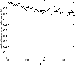
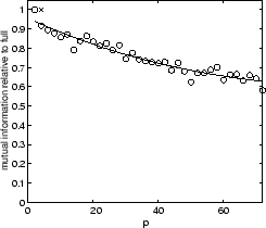
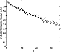
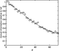
![]() . Figure 5.11 shows our results for the four
data-sets. Each plot in figure 5.11 shows the
relative mutual information (fraction of mutual information retained
as compared to the reference clustering on all objects and features)
as a function of the number of partitions. We fix the sum of the
number of objects in all partitions to be double the number
of objects (
. Figure 5.11 shows our results for the four
data-sets. Each plot in figure 5.11 shows the
relative mutual information (fraction of mutual information retained
as compared to the reference clustering on all objects and features)
as a function of the number of partitions. We fix the sum of the
number of objects in all partitions to be double the number
of objects (![]() ).
Within each plot,
).
Within each plot, ![]() ranges from 2 to 72 and each ODC result is
marked with a `
ranges from 2 to 72 and each ODC result is
marked with a `![]() '.
The reference point for unpartitioned data is marked by
`
'.
The reference point for unpartitioned data is marked by
`![]() ' at (1,1). For each of the plots, we fitted a sigmoid function to
summarize the behavior of ODC for that scenario.
' at (1,1). For each of the plots, we fitted a sigmoid function to
summarize the behavior of ODC for that scenario.
Clearly, there is a tradeoff in the number of partitions versus
quality. As ![]() approaches
approaches ![]() , each clusterer only
receives a single point and can make no reasonable grouping.
For example, in the YAHOO case, for
, each clusterer only
receives a single point and can make no reasonable grouping.
For example, in the YAHOO case, for ![]() processing on
16 partitions still retains around
90% (80%) of the full quality. For less complex data-sets,
such as 2D2K, combining 16 partial partitionings (
processing on
16 partitions still retains around
90% (80%) of the full quality. For less complex data-sets,
such as 2D2K, combining 16 partial partitionings (![]() )
still yields 90% of the quality. In fact, 2D2K can be clustered in 72 partitions at 80% quality.
Also, we observed that for easier data-sets there is a smaller absolute loss in quality for more partitions
)
still yields 90% of the quality. In fact, 2D2K can be clustered in 72 partitions at 80% quality.
Also, we observed that for easier data-sets there is a smaller absolute loss in quality for more partitions ![]() .
.
Regarding our proposed techniques, all three algorithms achieved similar ANMI scores without significant differences for 8D5K, PENDIG, and YAHOO. HGPA had some instabilities for the 2D2K data-set delivering inferior consensus clusterings compared to MCLA and CSPA.
In general, we believe the loss in quality with ![]() has two main
causes. First, through the reduction of considered pairwise
relations, the problem is simplified as speedup increases. At some
point too much relationship information is lost to reconstruct the
original clusters.
The second factor is related to the balancing constraints used by the
graph partitioner in the inner loop: the sampling strategies cannot
maintain the balancing, so enforcing them in clustering hurts quality.
A relaxed inner loop clusterer might improve results.
has two main
causes. First, through the reduction of considered pairwise
relations, the problem is simplified as speedup increases. At some
point too much relationship information is lost to reconstruct the
original clusters.
The second factor is related to the balancing constraints used by the
graph partitioner in the inner loop: the sampling strategies cannot
maintain the balancing, so enforcing them in clustering hurts quality.
A relaxed inner loop clusterer might improve results.
|
Distributed clustering using a cluster ensemble is particularly
useful when the inner loop clustering algorithm has superlinear
complexity (![]() ) and a fast consensus function (such as MCLA and
HGPA) is used.
In this case, additional speedups can be obtained
through distribution of objects.
Let us assume that the inner loop clusterer has a complexity of
) and a fast consensus function (such as MCLA and
HGPA) is used.
In this case, additional speedups can be obtained
through distribution of objects.
Let us assume that the inner loop clusterer has a complexity of
![]() (e.g., similarity-based approaches or efficient agglomerative
clustering) and one uses only MCLA and HGPA in the supra-consensus
function.5.13We define speedup as the computation time for the full
clustering divided by the time when using the ODC approach.
The overhead for the MCLA and HGPA consensus functions grows linear in
(e.g., similarity-based approaches or efficient agglomerative
clustering) and one uses only MCLA and HGPA in the supra-consensus
function.5.13We define speedup as the computation time for the full
clustering divided by the time when using the ODC approach.
The overhead for the MCLA and HGPA consensus functions grows linear in
![]() and is negligible compared to the
and is negligible compared to the ![]() clustering. Hence the
sequential speedup is approximately
clustering. Hence the
sequential speedup is approximately
![]() .
Each partition can be clustered without any communication on a
separate processor. At integration time only the
.
Each partition can be clustered without any communication on a
separate processor. At integration time only the ![]() -dimensional label
vector (instead of e.g., the entire
-dimensional label
vector (instead of e.g., the entire
![]() similarity matrix)
has to be transmitted to the combiner. Hence, ODC does not only save
computation time, but also enables trivial
similarity matrix)
has to be transmitted to the combiner. Hence, ODC does not only save
computation time, but also enables trivial ![]() -fold parallelization.
Consequently the sequential speedup can be multiplied by
-fold parallelization.
Consequently the sequential speedup can be multiplied by ![]() if a
if a
![]() -processor computer is utilized:
-processor computer is utilized:
![]() .
An actual speedup (
.
An actual speedup (![]() ) will be reached for
) will be reached for ![]() in the
sequential or
in the
sequential or ![]() in the parallel case.
For example, when
in the parallel case.
For example, when ![]() and
and ![]() (which implies
(which implies ![]() ) the
computing time is approximately the same (
) the
computing time is approximately the same (![]() ) because each
partition is half the original size
) because each
partition is half the original size ![]() and consequently processed
in a quarter of the time. Since there are four partitions, ODC takes the
same time as the original processing.
In our experiments, using partitions from 2 to 72 yield
corresponding sequential (parallel)
speedups
from 0.5 (1) to 18 (1296). For example, 2D2K (YAHOO) can
be sped up 64-fold using 16 processors at 90% (80%) of the full
length quality. In fact, 2D2K can be clustered in less that
1/1000 of the original time at 80% quality.
and consequently processed
in a quarter of the time. Since there are four partitions, ODC takes the
same time as the original processing.
In our experiments, using partitions from 2 to 72 yield
corresponding sequential (parallel)
speedups
from 0.5 (1) to 18 (1296). For example, 2D2K (YAHOO) can
be sped up 64-fold using 16 processors at 90% (80%) of the full
length quality. In fact, 2D2K can be clustered in less that
1/1000 of the original time at 80% quality.