Next: OPOSSUM
Up: Relationship-based Clustering and Visualization
Previous: Motivation
Contents
Domain Specific Features and Similarity Space
Notation. Let  be the number of objects / samples / points (e.g.,
customers, documents, web-sessions) in the data and
be the number of objects / samples / points (e.g.,
customers, documents, web-sessions) in the data and  the number of
features (e.g., products, words, web-pages) for each sample
the number of
features (e.g., products, words, web-pages) for each sample
 with
with
 . Let
. Let  be the
desired number of clusters. The input data can be represented by a
be the
desired number of clusters. The input data can be represented by a
 data matrix
 with the
  -th column vector
representing the sample
.
-th column vector
representing the sample
.
 denotes the transpose of
. Hard clustering assigns a
label
denotes the transpose of
. Hard clustering assigns a
label
 to each -dimensional sample
, such that similar samples get the same label. In
general the labels are treated as nominals with no inherent order,
though in some cases, such as 1-dimensional SOMs, any top-down
recursive bisection approach as well as our proposed method, the
labeling contains extra ordering information. Let
to each -dimensional sample
, such that similar samples get the same label. In
general the labels are treated as nominals with no inherent order,
though in some cases, such as 1-dimensional SOMs, any top-down
recursive bisection approach as well as our proposed method, the
labeling contains extra ordering information. Let
 denote the set of all objects in the
  -th
cluster (
-th
cluster (
 ), with
 and
and
 .
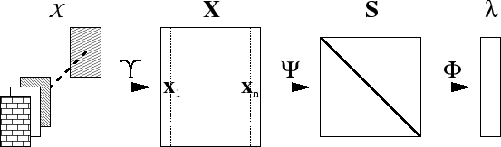
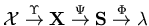
Figure 3.1 gives an overview of our relationship-based
clustering process from a set of raw object descriptions
.
Figure 3.1 gives an overview of our relationship-based
clustering process from a set of raw object descriptions
 (residing in input space
 ) via the vector
space description
(in feature space
) via the vector
space description
(in feature space
 ) and
relationship description
) and
relationship description
 (in similarity space
 ) to the cluster labels
 (in output
space
(in output
space
 ):
):
 .
For example in web-page clustering,
is a collection of
web-pages
.
For example in web-page clustering,
is a collection of
web-pages  with
. Extracting features
using
with
. Extracting features
using  yields
, the term frequencies of stemmed
words, normalized such that for all documents
yields
, the term frequencies of stemmed
words, normalized such that for all documents
 . Similarities are computed, using e.g., cosine-based similarity
  yielding the
 similarity matrix
. Finally, the cluster label vector
is
computed using a clustering function
similarity matrix
. Finally, the cluster label vector
is
computed using a clustering function  , such as
graph partitioning. In short, the basic process can be denoted as
, such as
graph partitioning. In short, the basic process can be denoted as
 .
.
Figure 3.1:
The relationship-based clustering framework.
|
|
Similarity Measures. In this dissertation, we prefer working in similarity space
rather than the original vector space in which the feature vectors
reside.
A similarity measure captures the relationship between two
-dimensional objects in a single number (using on the order of
the number of non-zero entries in the vectors or , at worst, computations). Once this is done, the
original high-dimensional space is not dealt with at all, we only work
in the transformed similarity space, and subsequent processing is
independent of .
A similarity measure ![$ \in [0,1]$](img177.png) captures how related two data-points
captures how related two data-points
 and
and
 are. It should be symmetric
(
are. It should be symmetric
(
 ), with
self-similarity
), with
self-similarity
 . However, in
general, similarity functions (respectively their distance function
equivalents
. However, in
general, similarity functions (respectively their distance function
equivalents
 , see below) do not obey the
triangle inequality.
An obvious way to compute similarity is through a suitable monotonic
and inverse function of a Minkowski (
, see below) do not obey the
triangle inequality.
An obvious way to compute similarity is through a suitable monotonic
and inverse function of a Minkowski ( ) distance,
  . Candidates
include
. Candidates
include
 and
and
 , the later being
preferable due to maximum likelihood properties (see chapter 4). Similarity can also be defined by the cosine
of the angle between two vectors:
, the later being
preferable due to maximum likelihood properties (see chapter 4). Similarity can also be defined by the cosine
of the angle between two vectors:
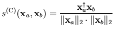 |
(3.1) |
Cosine similarity is widely used in text clustering because two
documents with the same proportions of term occurrences but different
lengths are often considered identical. In retail data such
normalization loses important information about the life-time customer
value, and we have recently shown that the extended Jaccard
similarity measure is more appropriate [SG00c]. For
binary features, the Jaccard coefficient [JD88] (also known as
the Tanimoto coefficient [DHS01]) measures the
ratio of the intersection of the product sets to the union of the
product sets corresponding to transactions
and
, each having binary (0/1) elements.
 |
(3.2) |
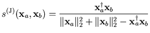
The extended Jaccard coefficient is also given by equation
3.2, but allows elements of
and
to be arbitrary positive real numbers. This coefficient
captures a vector-length-sensitive measure of similarity. However, it
is still invariant to scale (dilating
and
by the same factor does not change
 ). A detailed discussion of the
properties of various similarity measures can be found in
chapter 4.
Since, for general data distributions, one cannot avoid the `curse
of dimensionality', there is no similarity metric that is
optimal for all applications.
Rather, one needs to to determine an
appropriate measure for the given application, that captures the
essential aspects of the class of high-dimensional data distributions
being considered.
). A detailed discussion of the
properties of various similarity measures can be found in
chapter 4.
Since, for general data distributions, one cannot avoid the `curse
of dimensionality', there is no similarity metric that is
optimal for all applications.
Rather, one needs to to determine an
appropriate measure for the given application, that captures the
essential aspects of the class of high-dimensional data distributions
being considered.
Next: OPOSSUM
Up: Relationship-based Clustering and Visualization
Previous: Motivation
Contents
Alexander Strehl
2002-05-03