Vertex Weighted Graph Partitioning

We map the problem of clustering to partitioning a vertex weighted graph $\mathcal{G}$ into $k$ unconnected components of approximately equal size (as defined by the balancing constraint) by removing a minimal amount of edges. The objects to be clustered are viewed as a set of vertices $\mathcal{V} = \{\mathbf{x}_{1},\ldots,\mathbf{x}_{n}\}$. Two vertices $\mathbf{x}_a$ and $\mathbf{x}_b$ are connected with an undirected edge $(a,b) \in \mathcal{E}$ of positive weight given by the similarity $s(\mathbf{x}_a,\mathbf{x}_b)$. This defines the graph $\mathcal{G}=(\mathcal{V},\mathcal{E})$. An edge separator $\Delta \mathcal{E}$ is a set of edges whose removal splits the graph $\mathcal{G}$ into $k$ pair-wise unconnected components (sub-graphs) $\{ \mathcal{G}_{1},\ldots,\mathcal{G}_{k}\}$. All sub-graphs $\mathcal{G}_{\ell} =(\mathcal{V}_{\ell},\mathcal{E}_{\ell})$ have pairwise disjoint sets of vertices and edges. The edge separator for a particular partitioning includes all the edges that are not part of any sub-graph, or $\Delta \mathcal{E} = \left( \mathcal{E} \setminus ( \mathcal{E}_1 \cup \mathcal{E}_2 \cup \ldots \cup \mathcal{E}_k ) \right)$. The clustering task is thus to find an edge separator with a minimum sum of edge weights, that partitions the graph into $k$ disjoint pieces. The following equation formalizes this minimum cut objective:

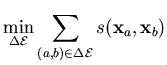$$\min_{\Delta \mathcal{E}} \sum_{(a,b) \in \Delta \mathcal{E}} s(\mathbf{x}_a,\mathbf{x}_b)$$ (3.3)

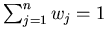
Without loss of generality, we can assume that the vertex weights $w_j$ are normalized to sum up to $1$: $\sum_{j=1}^n w_j = 1$. While striving for the minimum cut objective, the balancing constraint

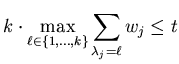$$k \cdot \max_{\ell \in \{1,\ldots,k\}} \sum_{\lambda_j = \ell} w_j \leq t$$ (3.4)

has to be fulfilled. The left hand side of the inequality is called the imbalance (the ratio of the biggest cluster in terms of cumulative normalized edge weight to the desired equal cluster-size $1/k$) and has a lower bound of 1. The balancing threshold $t$ enforces perfectly balanced clusters for $t=1$. In practice $t$ is often chosen to be slightly greater than 1 (e.g., we use $t=1.05$ for all our experiments which allows at most 5% of imbalance). Thus, in graph partitioning one has to essentially solve a constrained optimization problem. Finding such an optimal partitioning is an NP-hard problem [GJ79]. However, there are fast, heuristic algorithms for this widely studied problem. We experimented with the Kernighan-Lin (KL) algorithm, recursive spectral bisection, and multi-level $k$-way partitioning (METIS). The basic idea in KL [KL70] to dealing with graph partitioning is to construct an initial partition of the vertices either randomly or according to some problem-specific strategy. Then the algorithm sweeps through the vertices, deciding whether the size of the cut would increase or decrease if we moved this vertex $\mathbf{x}$ over to another partition. The decision to move $\mathbf{x}$ can be made in time proportional to its degree by simply counting whether more of $\mathbf{x}$'s neighbors are on the same partition as $\mathbf{x}$ or not. Of course, the desirable side for $\mathbf{x}$ will change if many of its neighbors switch, so multiple passes are likely to be needed before the process converges to a local optimum. In recursive bisection, a $k$-way split is obtained by recursively partitioning the graph into two subgraphs. Spectral bisection [PSL90,HL95] uses the eigenvector associated with the second smallest eigenvalue of the graph's Laplacian (Fiedler vector) [Fie75] for splitting. METIS [KK98a] handles multi-constraint multi-objective graph partitioning in three phases: (i) coarsening, (ii) initial partitioning, and (iii) refining. First a sequence of successively smaller and therefore coarser graphs is constructed through heavy-edge matching. Secondly, the initial partitioning is constructed using one out of four heuristic algorithms (three based on graph growing and one based on spectral bisection). In the third phase the coarsened partitioned graph undergoes boundary Kernighan-Lin refinement. In this last phase vertices are only swapped amongst neighboring partitions (boundaries). This ensures that neighboring clusters are more related than non-neighboring clusters. This ordering property is beneficial for visualization, as explained in subsection 3.6.1. In contrast, since recursive bisection computes a bisection of a subgraph at a time, its view is limited. Thus, it can not fully optimize the partition ordering and the global constraints. This renders it less effective for our purposes. Also, we found the multi-level partitioning to deliver the best partitionings as well as to be the fastest and most scalable of the three choices we investigated. Hence, METIS is used as the graph partitioner in OPOSSUM.