


Next: CLUSION: Cluster Visualization
Up: OPOSSUM
Previous: Vertex Weighted Graph Partitioning
Contents
Determining the Number of Clusters
Finding the `right' number of clusters  for a data-set is a
difficult and often ill-posed problem, since even for the same data-set, there can be several answers depending on the scale or
granularity one is interested in. In probabilistic approaches to
clustering, likelihood-ratios, Bayesian techniques and Monte Carlo
cross-validation are popular. In non-probabilistic methods, a
regularization approach, which penalizes for large , is often
adopted. If the data is labelled, then mutual information between
cluster and class labels can be used to determine the number of
clusters. Other metrics such as purity of clusters or entropy are of
less use as they are biased towards a larger number of clusters
(see chapter 4).
For transactional data, often the number is specified by the end-user
to be typically between 7 and 14 [BL97]. Otherwise, one can
employ a suitable heuristic to obtain an appropriate value of
during the clustering process.
This subsection describes how we find a desirable clustering, with
high overall cluster quality
for a data-set is a
difficult and often ill-posed problem, since even for the same data-set, there can be several answers depending on the scale or
granularity one is interested in. In probabilistic approaches to
clustering, likelihood-ratios, Bayesian techniques and Monte Carlo
cross-validation are popular. In non-probabilistic methods, a
regularization approach, which penalizes for large , is often
adopted. If the data is labelled, then mutual information between
cluster and class labels can be used to determine the number of
clusters. Other metrics such as purity of clusters or entropy are of
less use as they are biased towards a larger number of clusters
(see chapter 4).
For transactional data, often the number is specified by the end-user
to be typically between 7 and 14 [BL97]. Otherwise, one can
employ a suitable heuristic to obtain an appropriate value of
during the clustering process.
This subsection describes how we find a desirable clustering, with
high overall cluster quality
 and a small number of
clusters .
Our objective is to maximize intra-cluster similarity and minimize
inter-cluster similarity, given by
and a small number of
clusters .
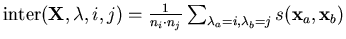
Our objective is to maximize intra-cluster similarity and minimize
inter-cluster similarity, given by
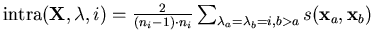 and
and
 ,
respectively, where
,
respectively, where  and
and  are cluster indices. Note that
intra-cluster similarity is undefined (0/0) for singleton
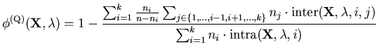
clusters. Hence, we define our quality measure
are cluster indices. Note that
intra-cluster similarity is undefined (0/0) for singleton
clusters. Hence, we define our quality measure
![$ \phi^{(\mathrm{Q})} \in [0,
1]$](img211.png) (
(
 in case of pathological / inverse clustering) based on
the ratio of weighted average inter-cluster to weighted average
intra-cluster similarity:
in case of pathological / inverse clustering) based on
the ratio of weighted average inter-cluster to weighted average
intra-cluster similarity:
 |
(3.5) |
 indicates that samples within the same cluster are on
average not more similar than samples from different clusters. On the
contrary,
indicates that samples within the same cluster are on
average not more similar than samples from different clusters. On the
contrary,
 describes a clustering where every pair of
samples from different clusters has the similarity of 0 and at least
one sample pair from the same cluster has a non-zero similarity. Note
that our definition of quality does not take the `amount of balance'
into account, since balancing is already observed fairly strictly by
the constraints in the graph partitioning step.
To achieve a high quality
as well as a low , the target
function
describes a clustering where every pair of
samples from different clusters has the similarity of 0 and at least
one sample pair from the same cluster has a non-zero similarity. Note
that our definition of quality does not take the `amount of balance'
into account, since balancing is already observed fairly strictly by
the constraints in the graph partitioning step.
To achieve a high quality
as well as a low , the target
function
![$ \phi^{(\mathrm{T})} \in [0,1]$](img216.png) is the product of the
quality
and a penalty term which works very well in practice.
If
is the product of the
quality
and a penalty term which works very well in practice.
If  and
and
 , then there
exists at least one clustering with no singleton clusters. The
penalized quality gives the penalized quality
, then there
exists at least one clustering with no singleton clusters. The
penalized quality gives the penalized quality
 and is defined as
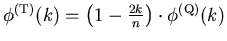 . A modest linear penalty was
chosen, since our quality criterion does not necessarily improve with
increasing (unlike e.g. the squared error criterion).
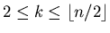
For large
. A modest linear penalty was
chosen, since our quality criterion does not necessarily improve with
increasing (unlike e.g. the squared error criterion).
For large  , we search for the optimal in the entire window from
 . In many cases, however, a forward search starting
at
. In many cases, however, a forward search starting
at  and stopping at the first down-tick of penalized quality while
increasing is sufficient.
Finally, a practical alternative, as exemplified by the experimental
results later, is to first over-cluster and then use the visualization
aid to combine clusters as needed (subsection 3.5.2).
and stopping at the first down-tick of penalized quality while
increasing is sufficient.
Finally, a practical alternative, as exemplified by the experimental
results later, is to first over-cluster and then use the visualization
aid to combine clusters as needed (subsection 3.5.2).
Next: CLUSION: Cluster Visualization
Up: OPOSSUM
Previous: Vertex Weighted Graph Partitioning
Contents
Alexander Strehl
2002-05-03