Web-document Clusters

In this subsection, we present results on documents from the Yahoo! news section. Each of the 2340 documents is characterized by a bag-of-words. The data is publicly available from ftp://ftp.cs.umn.edu/dept/users/boley/ (K1 series) and was used in [BGG$^+$99,SGM00]. The 20 original Yahoo! news categories are Business (B), Entertainment (no sub-category (E), art (a), cable (c), culture (cu), film (f), industry (i), media (m), multimedia (mm), music (mu), online (o), people (p), review (r), stage (s), television (t), variety (v)), Health (H), Politics (P), Sports (S), Technology (T) and correspond to the category labels 1,...,20, respectively. The raw 21839 $\times$ 2340 word-by-document matrix consists of the non-normalized occurrence frequencies of stemmed words, using Porter's suffix stripping algorithm [Fra92]. Pruning all words that occur less than 0.01 or more than 0.10 times on average because they are insignificant (e.g., haruspex) or too generic (e.g., new), respectively, results in $d=2903$. We call this data-set YAHOO (see also appendix A.5). Let us point out some worthwhile differences between clustering market-baskets and documents. Firstly, discrimination of vector length is no longer desired since customer life-time value matters but document length does not. Consequently, we use cosine similarity $s^{(\mathrm{C})}$ instead of extended Jaccard similarity $s^{(\mathrm{J})}$. Also, in document clustering we are less concerned about balancing, since there are usually no direct monetary costs of the actions derived from the clustering involved. As a consequence of this, we over-cluster first with sample-balanced OPOSSUM and then allow user guided merging of clusters through CLUSION. The YAHOO data-set is notorious for having some diffuse groups with overlaps among categories, a few categories with multi-modal distributions, etc. These aspects can be easily explored by looking at the class labels within each cluster, merging some clusters and then again visualizing the results. Figure 3.6 shows clusterings with three settings of $k$. For $k=10$ (figure 3.6(a)) most clusters are not dense enough, despite the fact that the first two clusters already seem like they should not have been split. After increasing to $k=40$ (figure 3.6(b)), CLUSION indicates that the clustering now has sufficiently compact clusters. Now, we successively merge pairs of highly related clusters until we obtain our final clustering with $k=20$ (figure 3.6(c)). The merging process is guided by inter-cluster similarity (e.g., bright off-diagonal regions) augmented by cluster-descriptions (e.g., related frequent words). In fact, in our graphical user interface of CLUSION merging is as easy as clicking on a selected off-diagonal region.

Figure 3.6: Comparison of various number of clusters $k$ for YAHOO news data: (a) under-clustering at $k=10$, (b) over-clustering at $k=40$, (c) good clustering through interactive split and merge using CLUSION at $k=20$. See color pictures in soft-copy for cluster boundaries.

(a)	(b)
(c)

Table 3.2: Cluster evaluations, their descriptive and discriminative terms (top) as well as the confusion matrix (bottom) for the YAHOO news example (see also figure 3.6(c)). For each cluster number $\mathcal{C}_{\ell}$ the dominant category $\mathcal{K}_{\hat{h}}$, purity $\phi^{(\mathrm{A})}$, and entropy $\phi^{(\mathrm{B})}$ are shown.

$\mathcal{C}_{\ell}$	$\mathcal{K}_{\hat{h}}$	$\phi^{(\mathrm{A})}$	$\phi^{(\mathrm{B})}$
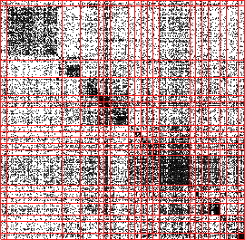
1	P	21.05%	0.73
2	H	91.48%	0.15
3	S	68.39%	0.40
4	P	52.84%	0.60
5	T	63.79%	0.39
6	o	57.63%	0.40
7	B	60.23%	0.48
8	f	37.93%	0.66
9	cu	50.85%	0.48
10	p	36.21%	0.56
11	f	67.80%	0.33
12	f	77.59%	0.31
13	r	47.28%	0.56
14	mu	44.07%	0.56
15	p	50.00%	0.50
16	mu	18.97%	0.71
17	p	55.08%	0.54
18	t	82.76%	0.24
19	f	38.79%	0.58
20	f	69.49%	0.36

top 3 descriptive terms

israel, teeth, dental

breast, smok, surgeri

smith, player, coach

republ, committe, reform

java, sun, card

apple, intel, electron

cent, quarter, rose

hbo, ali, alan

bestsell, weekli, hardcov

albert, nomin, winner

miramax, chri, novel

cast, shoot, indie

showbiz, sound, band

concert, artist, miami

notabl, venic, classic

fashion, sold, bbc

funer, crash, royal

househ, sitcom, timeslot

king, japanes, movi

weekend, ticket, gross

top 3 discriminative terms

mckinnei, prostat, weizman

symptom, protein, vitamin

hingi, touchdown, rodman

icke, veto, teamster

nader, wireless, lucent

pentium, ibm, compaq

dow, ahmanson, greenspan

phillip, lange, wendi

hardcov, chicken, bestsell

forcibl, meredith, sportscast

cusack, cameron, man

juliett, showtim, cast

dialogu, prodigi, submiss

bing, calla, goethe

stamp, skelton, espn

poetri, versac, worn

spencer, funer, manslaught

timeslot, slot, household

denot, winfrei, atop

weekend, gross, mimic

	B	E	a	c	cu	f	i	m	mm	mu	o	p	r	s	t	v	H	P	S	T
7	106	1	-	4	2	-	30	6	-	4	2	1	-	-	5	2	-	2	-	11
9	-	-	-	3	30	17	-	-	1	1	2	2	1	-	1	1	-	-	-	-
8	-	-	1	7	-	22	2	-	-	3	1	5	8	1	5	2	-	-	1	-
11	-	-	-	1	-	40	1	-	-	-	-	1	2	-	1	13	-	-	-	-
12	-	-	-	2	-	45	-	-	-	-	-	2	1	2	4	2	-	-	-	-
19	-	1	-	3	1	45	1	-	-	8	-	15	2	-	25	14	-	-	1	-
20	-	1	1	-	-	41	-	-	-	4	-	-	-	5	6	1	-	-	-	-
14	-	2	8	-	4	2	-	-	-	26	1	12	-	2	1	-	-	1	-	-
16	-	1	4	1	9	9	2	2	1	11	-	11	-	-	6	-	-	1	-	-
6	8	-	-	-	-	-	1	-	3	-	34	-	-	-	-	1	-	-	-	12
10	-	-	-	3	1	4	-	-	2	2	1	21	2	-	20	2	-	-	-	-
15	-	-	2	1	5	13	-	-	-	4	2	29	-	-	2	-	-	-	-	-
17	-	1	-	2	6	5	1	6	-	12	1	65	3	-	12	4	-	-	-	-
13	-	-	1	1	9	22	6	1	3	33	9	58	139	7	2	3	-	-	-	-
18	-	-	1	2	-	1	-	-	-	-	-	2	-	-	48	4	-	-	-	-
2	2	-	-	2	1	1	1	-	1	1	3	5	-	-	6	-	483	5	17	-
1	3	2	2	1	-	4	-	1	-	4	-	10	-	-	5	-	11	12	2	-
4	14	-	4	7	5	2	15	5	-	6	3	6	-	1	12	2	-	93	1	-
3	1	-	-	1	1	5	10	-	3	5	-	3	-	-	23	3	-	-	119	-
5	8	-	-	3	-	-	-	-	-	1	6	-	-	-	3	-	-	-	-	37

Table 3.2(top) shows cluster evaluations, their descriptive and discriminative word stems. Each cluster ( $\mathcal{C}_{\ell}$) is evaluated using the dominant category ( $\mathcal{K}_{\hat{h}}$), purity ( $\phi^{(\mathrm{A})}$), and entropy ( $\phi^{(\mathrm{B})}$). Let $n_{\ell}^{(h)}$ denote the number of objects in cluster $\mathcal{C}_{\ell}$ that are classified to be in category $h$ as given by the original Yahoo! categorization. Cluster $\mathcal{C}_{\ell}$'s purity can be defined as

$$\phi^{(\mathrm{A})} (\mathcal{C}_{\ell}) = \frac{1}{n_{\ell}} \max_h (n_{\ell}^{(h)}) .$$ (3.9)

Purity can be interpreted as the classification rate under the assumption that all samples of a cluster are predicted to be members of the actual dominant class for that cluster. Alternatively, we also use [0,1]-normalized entropy, which is defined for a problem with $g$ categories as

$$\phi^{(\mathrm{B})} (\mathcal{C}_{\ell}) = - \sum_{h=1}^g \frac{... ...l}^{(h)}}{n_{\ell}} \log_g \left( \frac{n_{\ell}^{(h)}}{n_{\ell}} \right) .$$ (3.10)

Entropy is a more comprehensive measure than purity since rather than just considering the number of objects `in' and `not in' the most frequent category, it considers the entire distribution. Table 3.2(bottom) gives the complete confusion matrix, which indicates how clusters and categories are related. Note that neither category nor prior distribution information is used during the unsupervised clustering process. In fact, the clustering is very good. It is much better than the original categorization in terms of edge cut and similarity lift, and it provides a much better grouping when only word frequencies are looked at. The evaluation metrics serve the purpose of validating our results capture relevant categorizations. However, their importance for our purpose is limited since we are solving a clustering problem and not a classification problem. The largest and best cluster is cluster $\mathcal{C}_2$ with 483 out of 528 documents being from the health cluster. Health related documents show a very distinct set of words and can, hence, be nicely separated. Small and not well distinguished categories have been put together with other documents (For example, the arts category has mostly been absorbed by the music category to form clusters 14 and 16.). This is inevitable since the 20 categories vary widely in size from 9 to 494 documents while the clusters OPOSSUM provides are much more balanced (from 58 to 528 documents per cluster).