Retail Market-basket Clusters

First, we will show clusters in a real retail transaction database of 21672 customers of a drugstore^3.4. For the purpose of the experiments in this chapter, we randomly selected 2500 customers. The total number of transactions (cash register scans) for these customers is 33814 over a time interval of three months. We rolled up the product hierarchy once to obtain 1236 different products purchased. 15% of the total revenue is contributed by the single item Financial-Depts (on site financial services such as check cashing and bill payment) which was removed because it was too common. 473 of these products accounted for less than $25 each in toto and were dropped. The remaining $n=2466$ customers (34 customers had empty baskets after removing the irrelevant products) with their $d=762$ features compose the RETAIL data-set. Appendix A.4 gives exemplary transactions and illustrates Zipf-like distributions found in the data. The customers in RETAIL were clustered using OPOSSUM. The extended price was used as the feature entries to represent purchased quantity weighted according to price. In this customer clustering case study we set $k=20$. In this application domain, the number of clusters is often predetermined by marketing considerations such as advertising industry standards, marketing budgets, marketers ability to handle multiple groups, and the cost of personalization. In general, a reasonable value of $k$ can be obtained using heuristics (subsection 3.3.3). OPOSSUM's results for this example are obtained with a 1.7 GHz Pentium 4 PC with 512 MB RAM in approximately 35 seconds ($\sim$30s file I/O, 2.5s similarity computation, 0.5s conversion to integer weighted graph, 0.5s graph partitioning). 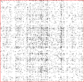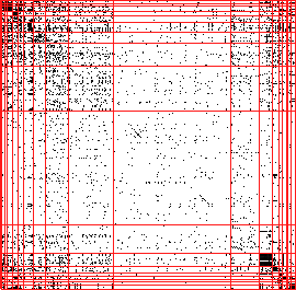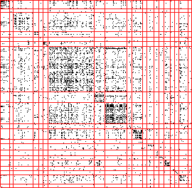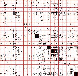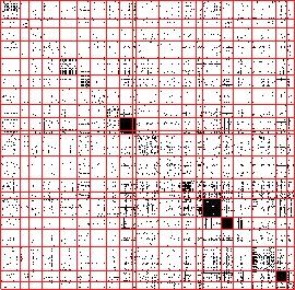Figures 3.4 and 3.5 show the extended Jaccard similarity matrix (83% sparse) using CLUSION in six scenarios: 3.4(a) original (randomly) ordered matrix, 3.4(b) seriated using Euclidean $k$-means, 3.4(c) using SOM, 3.4(d) using standard Jaccard $k$-means, 3.5(a) using extended Jaccard sample balanced OPOSSUM, 3.5(b) using value balanced OPOSSUM clustering. Customer and revenue ranges are given below each image. In figure 3.4(a), (b), (c), and (d) clusters are neither compact nor balanced. In figure 3.5(a) and (b) clusters are much more compact, even though there is the additional constraint that they be balanced, based on equal number of customers and equal revenue metrics, respectively. Below each CLUSION visualization, the ranges of numbers of customers and revenue totals in $ amongst the 20 cluster are given to indicate balancedness. We also experimented with minimum distance agglomerative clustering but this resulted in 19 singletons and 1 cluster with 2447 customers so we did not bother including this approach. Clearly, $k$-means in the original feature space, the standard clustering algorithm, does not perform well at all (figure 3.4(b)). The SOM after 100000 epochs performs slightly better (figure 3.4(c)) but is outperformed by the standard Jaccard $k$-means (figure 3.4(d)) which is adopted to similarity space by using $\sqrt{-\log(s^{(\mathrm{J})})}$ as distances (see chapter 4). As the relationship-based CLUSION shows, OPOSSUM (figure 3.5(a),(b)) gives more compact (better separation of on- and off-diagonal regions) and well balanced clusters as compared to all other techniques. For example, looking at standard Jaccard $k$-means, the clusters contain between 48 and 597 customers contributing between $608 and $70443 to revenue^3.5. Thus the clusters may not be of comparable importance from a marketing standpoint. Moreover clusters are hardly compact: Darkness is only slightly stronger in the on-diagonal regions in figure 3.4(d). All visualizations have been histogram equalized for printing purposes. However, they are still much better observed by browsing interactively on a computer screen.

Figure 3.4: Visualizing partitioning drugstore customers from RETAIL data-set into 20 clusters. Relationship visualizations using CLUSION: (a) original (randomly) ordered similarity matrix, (b) seriated or partially reordered using Euclidean $k$-means, (c) using SOM, (d) using standard Jaccard $k$-means. Customer and revenue ranges are given below each image. See also figure 3.5.

(a) 2466 customers, $126899 revenue	(b) [$1 - $1645], [$52 - $78480]
(c) [4 - 978], [$1261 - $12162]	(d) [48 - 597], [$608 - $70443]

Figure 3.5: Visualizing partitioning drugstore customers from RETAIL data-set into 20 clusters. Relationship visualizations using CLUSION: (a) using extended Jaccard sample balanced OPOSSUM, (b) using value balanced OPOSSUM clustering. Customer and revenue ranges are given below each image. In figure 3.4(a), (b), (c), and (d) clusters are neither compact nor balanced. In figure 3.5(a) and (b) clusters are much more compact, even thoughthere is the additional constraint that they be balanced, based on equal number of customers and equal revenue metrics, respectively.

(a) [122 - 125], [$1624 - $14361]	(b) [28 - 203], [$6187 - $6609]

A very compact and useful way of profiling a cluster is to look at their most descriptive and their most discriminative features. For market-basket data, this can be done by looking at a cluster's highest revenue products and the most unusual revenue drivers (e.g., products with highest revenue lift). Revenue lift is the ratio of the average spending on a product in a particular cluster to the average spending in the entire data-set.

Table 3.1: List of descriptive (top) and discriminative products (bottom) dominant in each of the 20 value balanced clusters obtained from the RETAIL data (see also figure 3.5(b)). For each item the average amount of $ spent in this cluster and the corresponding lift is given.

$\mathcal{C}_{\ell}$	top product	$	lift	sec. product	$	lift	third product	$	lift
1	bath gift packs	3.44	7.69	hair growth m	0.90	9.73	boutique island	0.81	2.61
2	smoking cessati	10.15	34.73	tp canning item	2.04	18.74	blood pressure	1.69	34.73
3	vitamins other	3.56	12.57	tp coffee maker	1.46	10.90	underpads hea	1.31	16.52
4	games items 180	3.10	7.32	facial moisturi	1.80	6.04	tp wine jug ite	1.25	8.01
5	batt alkaline i	4.37	7.27	appliances item	3.65	11.99	appliances appl	2.00	9.12
6	christmas light	8.11	12.22	appliances hair	1.61	7.23	tp toaster/oven	0.67	4.03
7	christmas food	3.42	7.35	christmas cards	1.99	6.19	cold bronchial	1.91	12.02
8	girl toys/dolls	4.13	12.51	boy toys items	3.42	8.20	everyday girls	1.85	6.46
9	christmas giftw	12.51	12.99	christmas home	1.24	3.92	christmas food	0.97	2.07
10	christmas giftw	19.94	20.71	christmas light	5.63	8.49	pers cd player	4.28	70.46
11	tp laundry soap	1.20	5.17	facial cleanser	1.11	4.15	hand&body thera	0.76	5.55
12	film cameras it	1.64	5.20	planners/calend	0.94	5.02	antacid h2 bloc	0.69	3.85
13	tools/accessori	4.46	11.17	binders items 2	3.59	10.16	drawing supplie	1.96	7.71
14	american greeti	4.42	5.34	paperback items	2.69	11.04	fragrances op	2.66	12.27
15	american greeti	5.56	6.72	christmas cards	0.45	2.12	basket candy it	0.44	1.45
16	tp seasonal boo	10.78	15.49	american greeti	0.98	1.18	valentine box c	0.71	4.08
17	vitamins e item	1.76	6.79	group stationer	1.01	11.55	tp seasonal boo	0.99	1.42
18	halloween bag c	2.11	6.06	basket candy it	1.23	4.07	cold cold items	1.17	4.24
19	hair clr perman	12.00	16.76	american greeti	1.11	1.34	revlon cls face	0.83	3.07
20	revlon cls face	7.05	26.06	hair clr perman	4.14	5.77	headache ibupro	2.37	12.65

$\mathcal{C}_{\ell}$	top product	$	lift	sec. product	$	lift	third product	$	lift
1	action items 30	0.26	15.13	tp video comedy	0.19	15.13	family items 30	0.14	11.41
2	smoking cessati	10.15	34.73	blood pressure	1.69	34.73	snacks/pnts nut	0.44	34.73
3	underpads hea	1.31	16.52	miscellaneous k	0.53	15.59	tp irons items	0.47	14.28
4	acrylics/gels/w	0.19	11.22	tp exercise ite	0.15	11.20	dental applianc	0.81	9.50
5	appliances item	3.65	11.99	housewares peg	0.13	9.92	tp tarps items	0.22	9.58
6	multiples packs	0.17	13.87	christmas light	8.11	12.22	tv's items 6	0.44	8.32
7	sleep aids item	0.31	14.61	kava kava items	0.51	14.21	tp beer super p	0.14	12.44
8	batt rechargeab	0.34	21.82	tp razors items	0.28	21.82	tp metal cookwa	0.39	12.77
9	tp furniture it	0.45	22.42	tp art&craft al	0.19	13.77	tp family plan,	0.15	13.76
10	pers cd player	4.28	70.46	tp plumbing ite	1.71	56.24	umbrellas adult	0.89	48.92
11	cat litter scoo	0.10	8.70	child acetamino	0.12	7.25	pro treatment i	0.07	6.78
12	heaters items 8	0.16	12.91	laverdiere ca	0.14	10.49	ginseng items 4	0.20	6.10
13	mop/broom lint	0.17	13.73	halloween cards	0.30	12.39	tools/accessori	4.46	11.17
14	dental repair k	0.80	38.17	tp lawn seed it	0.44	35.88	tp telephones/a	2.20	31.73
15	gift boxes item	0.10	8.18	hearing aid bat	0.08	7.25	american greeti	5.56	6.72
16	economy diapers	0.21	17.50	tp seasonal boo	10.78	15.49	girls socks ite	0.16	12.20
17	tp wine 1.5l va	0.17	15.91	group stationer	1.01	11.55	stereos items 2	0.13	10.61
18	tp med oint liq	0.10	8.22	tp dinnerware i	0.32	7.70	tp bath towels	0.12	7.28
19	hair clr perman	12.00	16.76	covergirl imple	0.14	11.83	tp power tools	0.25	10.89
20	revlon cls face	7.05	26.06	telephones cord	0.56	25.92	ardell lashes i	0.59	21.87

In table 3.1 the top three descriptive and discriminative products for the customers in the 20 value balanced clusters are shown (see also figure 3.5(b)). Customers in cluster $\mathcal{C}_2$, for example, mostly spent their money on smoking cessation gum ($10.15 on average). Interestingly, while this is a 35-fold average spending on smoking cessation gum, these customers also spend 35 times more on blood pressure related items, peanuts and snacks. Do these customers lead an unhealthy lifestyle and are eager to change? Cluster $\mathcal{C}_{15}$, which can be seen to be highly compact cluster of Christmas shoppers characterized by greeting card and candy purchases. Note that OPOSSUM had an extra constraint that clusters should be of comparable value. This may force a larger natural cluster to split, as may be the case causing the similar clusters $\mathcal{C}_{9}$ and $\mathcal{C}_{10}$. Both are Christmas gift shoppers (table 3.1(top)), cluster $\mathcal{C}_{9}$ are the moderate spenders and cluster $\mathcal{C}_{10}$ are the big spenders, as cluster $\mathcal{C}_{10}$ is much smaller with equal revenue contribution (figure 3.5(b)). Our hunch is reinforced by looking at figure 3.5(b).