In this section, we present and compare the results of the eleven
approaches on the four document data-sets. Clustering quality is
understood in terms of mutual information and balance.
For each data-set we set the number of clusters ![]() to be twice the
number of categories
to be twice the
number of categories ![]() , except for the REUT data-set where we
used
, except for the REUT data-set where we
used ![]() since there are many small categories.
Using a greater number of clusters than classes
allows multi-modal distributions for each class. For example, in
an XOR like problem, there are two classes, but four
clusters.
since there are many small categories.
Using a greater number of clusters than classes
allows multi-modal distributions for each class. For example, in
an XOR like problem, there are two classes, but four
clusters.
Let us first look at a representative result to illustrate the
behavior of some algorithms and our evaluation methodology.
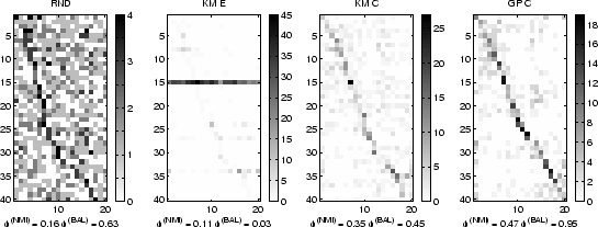
In figure 4.3, confusion matrices illustrating quality
differences of RND, KM E, KM C, and GP C approaches on a sample of 800
documents from N20 are shown.
The horizontal and vertical axis correspond to the categories and
clusters, respectively. Clusters are sorted in increasing order of
dominant category. Entries indicate the number
![]() of
documents in cluster
of
documents in cluster ![]() and category
and category ![]() by darkness. Expectedly,
random partitioning RND results in indiscriminating clusters with a
mutual information score
by darkness. Expectedly,
random partitioning RND results in indiscriminating clusters with a
mutual information score
![]() . The purity
score
. The purity
score
![]() indicates that on average the
dominant category contributes 16% of the objects in a
cluster. However, since labels are drawn from a uniform distribution,
cluster sizes are somewhat balanced with
indicates that on average the
dominant category contributes 16% of the objects in a
cluster. However, since labels are drawn from a uniform distribution,
cluster sizes are somewhat balanced with
![]() . KM E delivers one large cluster (cluster 15) and many small
clusters with
. KM E delivers one large cluster (cluster 15) and many small
clusters with
![]() . This strongly
imbalanced clustering is characteristic for KM E on high-dimensional
sparse data and is problematic because it usually defeats certain
application specific purposes such as browsing. It also results in
sub-random quality
. This strongly
imbalanced clustering is characteristic for KM E on high-dimensional
sparse data and is problematic because it usually defeats certain
application specific purposes such as browsing. It also results in
sub-random quality
![]() (
(
![]() ). KM C results are good. A
`diagonal' can be clearly seen in the confusion matrix. This
indicates that the clusters align with the ground truth categorization
which is reflected by an overall mutual information
). KM C results are good. A
`diagonal' can be clearly seen in the confusion matrix. This
indicates that the clusters align with the ground truth categorization
which is reflected by an overall mutual information
![]() (
(
![]() ). Balancing is good as well with
). Balancing is good as well with
![]() . GP C exceeds KM C in both aspects with
. GP C exceeds KM C in both aspects with
![]() (
(
![]() ) as well as balance
) as well as balance
![]() . The `diagonal' is stronger and
clusters are very balanced.
. The `diagonal' is stronger and
clusters are very balanced.
|
The rest of the results are given in summarized form instead of the more detailed treatment in the example above, since the comparative trends are very clear even at this macro level. Some examples of detailed confusion matrices and pairwise t-tests can be found in our earlier work [SGM00].
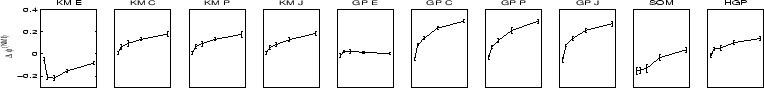
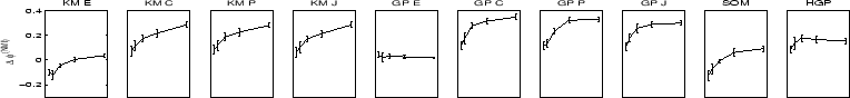
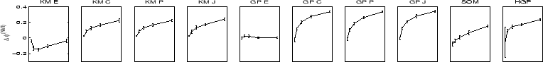
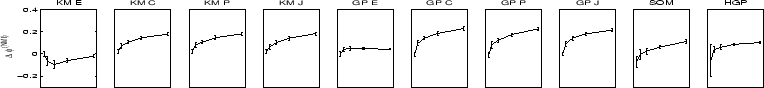
For a systematic comparison, ten experiments were performed for each
of the random samples of sizes 50, 100, 200, 400, and 800.
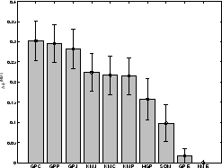
Figure 4.4 shows performance curves in terms of
(relative) mutual information comparing 10 algorithms on 4 data
sets. Each curve shows the difference
![]() in mutual information-based quality
in mutual information-based quality
![]() compared to random partitioning for 5 sample
sizes (at 50, 100, 200, 400, and 800). Error bars indicate
compared to random partitioning for 5 sample
sizes (at 50, 100, 200, 400, and 800). Error bars indicate ![]() 1
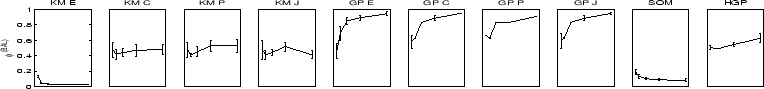
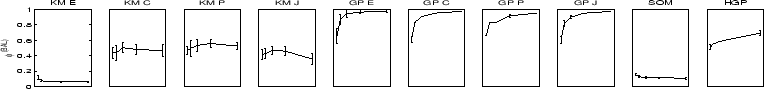
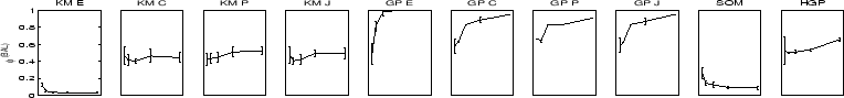
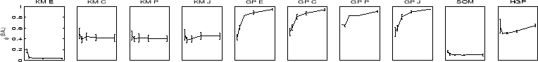
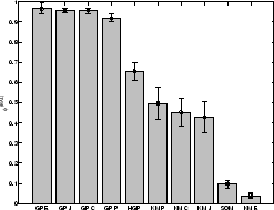
standard deviations over 10 experiments. Figure
4.5 shows quality in terms of balance for 4 data
sets in combination with 10 algorithms. Each curve shows the cluster
balance
1
standard deviations over 10 experiments. Figure
4.5 shows quality in terms of balance for 4 data
sets in combination with 10 algorithms. Each curve shows the cluster
balance
![]() for 5 sample sizes (again at 50,
100, 200, 400, and 800). Error bars indicate
for 5 sample sizes (again at 50,
100, 200, 400, and 800). Error bars indicate ![]() 1 standard
deviations over 10 experiments. Figure 4.6
summarizes the results on all four data-sets at the highest sample
size level (
1 standard
deviations over 10 experiments. Figure 4.6
summarizes the results on all four data-sets at the highest sample
size level (![]() ). We also conducted pairwise t-tests at
). We also conducted pairwise t-tests at ![]() to
assure differences in average performance are significant. For
illustration and brevity, we chose to show mean performance with
standard variation bars rather than the t-test results (see our
previous work [SGM00]).
to
assure differences in average performance are significant. For
illustration and brevity, we chose to show mean performance with
standard variation bars rather than the t-test results (see our
previous work [SGM00]).
First, we look at quality in terms of mutual information (figures
4.4, 4.6(a)). With increasing
sample size ![]() , the quality of clusterings tends to
improve. Non-metric (cosine, correlation, Jaccard) graph partitioning
approaches work best on text data (
, the quality of clusterings tends to
improve. Non-metric (cosine, correlation, Jaccard) graph partitioning
approaches work best on text data (
![]() )
followed by non-metric
)
followed by non-metric ![]() -means
approaches. Clearly, a non-metric e.g., dot-product-based similarity
measure is necessary for good quality. Due to the conservative
normalization, depending on the given data-set the maximum obtainable
mutual information (for a perfect classifier!) tends to be around
0.8 to 0.9. A mutual information-based quality around 0.4 and 0.5
(which is approximately 0.3 to 0.4 better than random at
-means
approaches. Clearly, a non-metric e.g., dot-product-based similarity
measure is necessary for good quality. Due to the conservative
normalization, depending on the given data-set the maximum obtainable
mutual information (for a perfect classifier!) tends to be around
0.8 to 0.9. A mutual information-based quality around 0.4 and 0.5
(which is approximately 0.3 to 0.4 better than random at ![]() ) is
an excellent result.4.7Hypergraph partitioning constitutes the third tier. Euclidean
techniques including SOM perform rather poorly. Surprisingly, the SOM
still delivers significantly better than random results despite the
limited expressiveness of the implicitly used Euclidean distances.
The success of SOM is explained with the fact that the Euclidean
distance becomes locally meaningful once the cell-centroids are locked
onto a good cluster.
) is
an excellent result.4.7Hypergraph partitioning constitutes the third tier. Euclidean
techniques including SOM perform rather poorly. Surprisingly, the SOM
still delivers significantly better than random results despite the
limited expressiveness of the implicitly used Euclidean distances.
The success of SOM is explained with the fact that the Euclidean
distance becomes locally meaningful once the cell-centroids are locked
onto a good cluster.
All approaches behaved consistently over the four data-sets with only slightly different scale caused by the different data-sets' complexities. The performance was best on YAHOO and WEBKB followed by N20 and REUT. Interestingly, the gap between GP and KM techniques is wider on YAHOO than on WEBKB. The low performance on REUT is probably due to the high number of classes (82) and their widely varying sizes.
In order to assess which approaches are more suitable for a particular
amount of objects ![]() , we also looked for intersects in the
performance curves of the top algorithms (non-metric GP and KM,
HGP).4.8In our experiments, the curves do not intersect indicating that
ranking of the top performers does not change in the range of data-set
sizes considered.
, we also looked for intersects in the
performance curves of the top algorithms (non-metric GP and KM,
HGP).4.8In our experiments, the curves do not intersect indicating that
ranking of the top performers does not change in the range of data-set
sizes considered.
In terms of balance (figures 4.5,
4.6(b)) the advantages of graph partitioning are
clear. Graph partitioning explicitly tries to achieve balanced
clusters (
![]() ). The second
tier is hypergraph partitioning which is also a balanced technique
(
). The second
tier is hypergraph partitioning which is also a balanced technique
(
![]() ) followed by non-metric
) followed by non-metric
![]() -means approaches (
-means approaches (
![]() ).
Poor balancing is shown by SOM and Euclidean
).
Poor balancing is shown by SOM and Euclidean ![]() -means
(
-means
(
![]() ). Interestingly,
balancedness does not change significantly for the
). Interestingly,
balancedness does not change significantly for the ![]() -means-based
approaches as the number of samples
-means-based
approaches as the number of samples ![]() increases. Graph partitioning
based approaches quickly approach perfect balancing as would be
expected since they are explicitly designed to do so.
increases. Graph partitioning
based approaches quickly approach perfect balancing as would be
expected since they are explicitly designed to do so.
Non-metric graph partitioning is significantly better in terms of mutual information as well as in balance. There is no significant difference in performance amongst the non-metric similarity measures using cosine, correlation, and extended Jaccard. Euclidean distance based approaches do not perform better than random clustering.
|
|
|