Discussion and Comparison

Let us first take a look at the worst case time complexity of the proposed algorithms. Assuming quasi-linear (hyper-)graph partitioners such as (H)METIS, CSPA is $O(n^2 k r)$, HGPA is $O(n k r)$, and MCLA is $O(n k^2 r^2)$. The fastest is HGPA, closely followed by MCLA since $k$ tends to be small. CSPA is the slowest and can become intractable for large $n$.

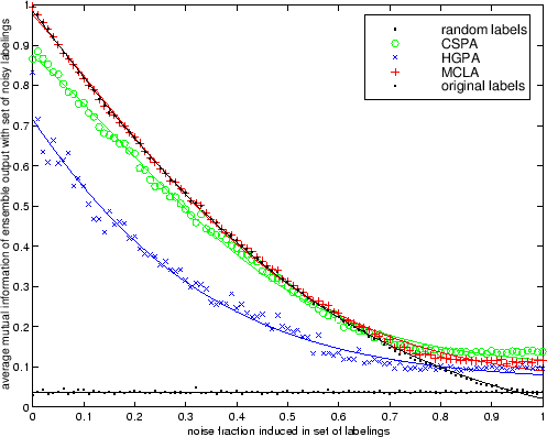
We performed a controlled experiment that allows us to compare the properties of the three proposed consensus functions. First, a we partition $n=500$ objects into $k=10$ groups at random to obtain the original clustering $\mathbf{\kappa}$.^5.6We duplicate this clustering $r=10$ times. Now in each of the 10 labelings, a fraction of the labels is replaced with random labels from a uniform distribution from 1 to $k$. Then, we feed the noisy labelings to the proposed consensus functions. The resulting combined labeling is evaluated in two ways. Firstly, we measure the normalized objective function $\phi^{(\mathrm{ANMI})}(\mathbf{\Lambda},\mathbf{\lambda})$ of the ensemble output $\mathbf{\lambda}$ with all the individual labels in $\mathbf{\Lambda}$. Secondly, we measure the normalized mutual information of each consensus labeling with the original undistorted labeling using $\phi^{(\mathrm{NMI})}(\mathbf{\kappa},\mathbf{\lambda})$. For better comparison, we added a random label generator as a baseline method. Also, performance measures of a hypothetical consensus function that returns the original labels are included to illustrate maximum performance for low noise settings.^5.7

Figure 5.6: Comparison of consensus functions in terms of the objective function $\phi^{(\mathrm{ANMI})}(\mathbf{\Lambda},\mathbf{\lambda})$ (top) and in terms of their normalized mutual information with original labels $\phi^{(\mathrm{NMI})}(\mathbf{\kappa},\mathbf{\lambda})$ (bottom) for various noise levels. A fitted sigmoid (least squared error) is shown for all algorithms to show the trend.

Figure 5.6 shows the results. As noise increases, labelings share less information and thus maximum obtainable $\phi^{(\mathrm{ANMI})}(\mathbf{\Lambda},\mathbf{\lambda})$ decreases, and so does $\phi^{(\mathrm{ANMI})}(\mathbf{\Lambda},\mathbf{\lambda})$ for all techniques. HGPA performs the worst in this experiment, which we believe is due to the lacking provision of partially cut edges. MCLA retains more $\phi^{(\mathrm{ANMI})}(\mathbf{\Lambda},\mathbf{\lambda})$ than CSPA in presence of low to medium-high noise. Interestingly, in very high noise settings CSPA exceeds MCLA's performance. Note also that for such high noise settings the original labels have a lower average normalized mutual information $\phi^{(\mathrm{ANMI})}(\mathbf{\Lambda},\mathbf{\lambda})$. This is because the set of labels are almost completely random and the consensus algorithms recover whatever little common information is present whereas the original labeling is now almost fully unrelated. However, in most cases noise should not exceed 50% and MCLA seems to perform best in this simple controlled experiment. Figure 5.6 illustrates how well the algorithms can recover the true labeling in the presence of noise for robust clustering. As noise increases labelings share less information with the true labeling and thus the ensemble's $\phi^{(\mathrm{NMI})}(\mathbf{\kappa},\mathbf{\lambda})$ decreases. The ranking of the algorithms is the same using this measure with MCLA best, followed by CSPA, and HGPA worst. In fact, MCLA recovers the original labeling at up to 35% noise in this scenario! For less than 50%, the algorithms have the same ranking regardless of whether $\phi^{(\mathrm{ANMI})}(\mathbf{\Lambda},\mathbf{\lambda})$ or $\phi^{(\mathrm{NMI})}(\mathbf{\kappa},\mathbf{\lambda})$ is used. This indicates that our proposed objective function $\phi^{(\mathrm{ANMI})}(\mathbf{\Lambda},\mathbf{\lambda})$ is indeed appropriate since in real applications, $\kappa$ and, thus, $\phi^{(\mathrm{NMI})}(\mathbf{\kappa},\mathbf{\lambda})$ is not available.

This experiment indicates that MCLA should be best suited in terms of time complexity as well as quality. In the applications and experiments described in the following sections we observe that each combining method can result in a higher ANMI than the others for particular setups. In fact, we found that MCLA tends to be best in low noise/diversity settings and HGPA/CSPA tend to be better in high noise/diversity settings. This is because MCLA assumes that there are meaningful cluster correspondences which is more likely to be true when there is little noise and less diversity. Thus, it is useful to have all three methods.

Indeed, our objective function has an added advantage that it allows one to add a stage that selects the best consensus function without any supervision information, by simply selecting the one with the highest ANMI. So, for the experiments in this chapter, we first report the results of this `supra'-consensus function $\Gamma$, obtained by running all three algorithms, CSPA, HGPA and MCLA, and selecting the one with the greatest ANMI. Then, if there are significant differences or notable trends observed among the three algorithms, this further level of detail is described. Note that the supra-consensus function is completely unsupervised and avoids the problem of selecting the best combiner for a data-set beforehand.