Mixture Density Estimation

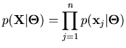
In statistical pattern recognition, the data is considered as a set of observations from a parametric probability distribution. [Fuk72,DH73]. In a two stage process, the parameters $\mathbf{\Theta}$ of the relevant distributions are learned and later applied to predict the behavior or origin of a new observation. In Maximum Likelihood (ML) estimation, the parameters $\hat{\mathbf{\Theta}}$ are chosen such that the probability of the observed samples $\mathbf{X}$ is maximized.

$$\hat{\mathbf{\Theta}} = \arg \max_{\mathbf{\Theta}} p(\mathbf{X} \vert \mathbf{\Theta})$$ (2.8)

Assuming that all samples are pairwise independent yields

$$p(\mathbf{X} \vert \mathbf{\Theta}) = \prod_{j = 1}^{n} p( \mathbf{x}_j \vert \mathbf{\Theta} )$$ (2.9)

Since each sample is drawn from a mixture distribution [EH81,Pri94] we have

$$p( \mathbf{x}_j \vert \mathbf{\Theta} ) = \sum_{\ell = 1}^{K} P(\... ...rt \mathbf{\Theta} , \omega_{\ell} ) ,\: \sum_{\ell=1}^{K} P(\omega_{\ell}) = 1$$ (2.10)

The cluster-conditional probability may be assumed to be a multivariate Gaussian which is defined as follows

$$p(\mathbf{x}_j \vert \mathbf{\Theta}, \omega_{\ell} ) = p(\mathbf... ...^{\dagger} \mathbf{\Sigma}_{\ell}^{-1} ( \mathbf{x}_j - \mathbf{\mu}_{\ell} ) }$$ (2.11)

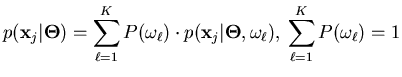
If there is domain knowledge or a desired behavior of the parameter $\mathbf{\Theta}$'s distribution, Bayes' learning should be used instead of the ML estimation.

$$\hat{\mathbf{\Theta}} = \arg \max_{\mathbf{\Theta}} p(\mathbf{\Theta} \vert \mathbf{X} )$$ (2.12)

Again, we expand $p(\mathbf{\Theta} \vert \mathbf{X} )$ using Bayes' rule.

$$p(\mathbf{\Theta} \vert \mathbf{X} ) = \frac{ p(\mathbf{\Theta}) \cdot p(\mathbf{X} \vert \mathbf{\Theta}) }{ p(\mathbf{X})}$$ (2.13)

The prior distribution $p(\mathbf{\Theta})$ can be known from the domain or estimated, $p(\mathbf{X} \vert \mathbf{\Theta})$ is the ML estimate as described above and $p(\mathbf{X})$ can be ignored for optimization purposes since it is constant in respect to $\mathbf{\Theta}$.

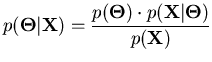
The learned distributions $p( \mathbf{x} \vert \mathbf{\Theta} , \omega_{\ell})$ can now be used for categorization and prediction of a sample's cluster label. The Bayes classifier is optimal in terms of prediction error, assuming that the distribution of the data is known precisely:

$$\lambda_j = \arg \max_{\ell \in \{1,\ldots,K\} } ( P(\omega_{\ell}) \cdot p( \mathbf{x}_j \vert \mathbf{\Theta} , \omega_{\ell} ) )$$ (2.14)

Often, using the log-likelihood (equation 2.15) instead of the actual probability values has advantages for optimization (e.g., convexity, products of very small probabilities which may be problematic for fixed precision numerics are avoided).

$$l(\mathbf{X}) = - \log p(\mathbf{X})$$ (2.15)

The theory behind statistical models is very well understood and explicit computations of error bounds are advantageous. Statistical formulations are advantageous for soft clustering problems with a moderate number of dimensions $d$. The very powerful Expectation-Maximization (EM) algorithm [DLR77] has been applied to $k$-means [FRB98]. However, these parametric models tend to impose structure on the data, that may not be there. The selected distribution family may not be really appropriate. In fact, high-dimensional data as found in data mining is distributed strongly non-Gaussian. Also, the number of parameters increases rapidly with $d$ so that the estimation problem becomes more and more ill-posed. Non-parametric models, like $v$-nearest-neighbor, have been found preferable in many tasks where a lot of data is available.