Visualization

The seriation of the similarity matrix, $\mathbf{S}'$, is very useful for visualization. Since the similarity matrix is 2-dimensional, it can be readily visualized as a gray-level image where a white (black) pixel corresponds to minimal (maximal) similarity of 0 (1). The darkness (gray level value) of the pixel at row $a$ and column $b$ increases with the similarity between the samples $\mathbf{x}_a$ and $\mathbf{x}_b$. When looking at the image it is useful to consider the similarity $s$ as a random variable taking values from 0 to 1. The expected similarity within cluster $\ell$ is thus represented by the average intensity within a square region with side length $n_{\ell}$, around the main diagonal of the matrix. The off-diagonal rectangular areas visualize the relationships between clusters. The brightness distribution in the rectangular areas yields insight towards the quality of the clustering and possible improvements. In order to make these regions apparent, thin red horizontal and vertical lines are used to show the divisions into the rectangular regions^3.3. Visualizing similarity space in this way can help to quickly get a feel for the clusters in the data. Even for a large number of points, a sense for the intrinsic number of clusters $k$ in a data-set can be gained.

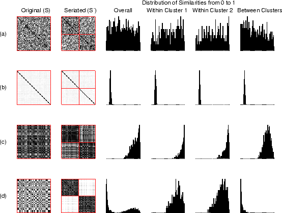
Figure 3.2: Illustrative CLUSION patterns in original order and seriated using optimal bipartitioning are shown in the left two columns. The right four columns show corresponding similarity distributions. In each example there are 50 objects: (a) no natural clusters (randomly related objects), (b) set of singletons (pairwise near orthogonal objects), (c) one natural cluster (uni-modal Gaussian), (d) two natural clusters (mixture of two Gaussians)

Figure 3.2 shows CLUSION output in four extreme scenarios to provide a feel for how data properties translate to the visual display. Without any loss of generality, we consider the partitioning of a set of objects into 2 clusters. For each scenario, on the left hand side the original similarity matrix $\mathbf{S}$ and the seriated version $\mathbf{S'}$ (CLUSION) for an optimal bipartitioning is shown. On the right hand side four histograms for the distribution of similarity values $s$, which range from 0 to 1, are shown. From left to right, we have plotted: distribution of $s$ over the entire data, within the first cluster, within the second cluster, and between first and second cluster. If the data is naturally clustered and the clustering algorithm is good, then the middle two columns of plots will be much more skewed to the right as compared to the first and fourth columns. In our visualization this corresponds to brighter off-diagonal regions and darker block diagonal regions in $\mathbf{S'}$ as compared to the original $\mathbf{S}$ matrix. The proposed visualization technique is quite powerful and versatile. In figure 3.2(a) the chosen similarity behaves randomly. Consequently, no strong visual difference between on- and off-diagonal regions can be perceived with CLUSION in $\mathbf{S'}$. It indicates clustering is ineffective which is expected since there is no structure in the similarity matrix. Figure 3.2(b) is based on data consisting of pair-wise almost equi-distant singletons. Clustering into two groups still renders the on-diagonal regions very bright suggesting more splits. In fact, this will remain unchanged until each data-point is a cluster by itself, thus, revealing the singleton character of the data. For monolithic data (figure 3.2(c)), many strong similarities are indicated by an almost uniformly dark similarity matrix $\mathbf{S}$. Splitting the data results in dark off-diagonal regions in $\mathbf{S'}$. A dark off-diagonal region suggests that the clusters in the corresponding rows and columns should be merged (or not be split in the first place). CLUSION indicates that this data is actually one large cluster. In figure 3.2(d), the gray-level distribution of $\mathbf{S}$ exposes bright as well as dark pixels, thereby recommending it should be split. In this case, $k=2$ apparently is a very good choice (and the clustering algorithm worked well) because in $\mathbf{S'}$ on-diagonal regions are uniformly dark and off-diagonal regions are uniformly bright. This induces an intuitive mining process that guides the user to the `right' number of clusters. Too small a $k$ leaves the on-diagonal regions inhomogeneous. On the contrary, growing $k$ beyond the natural number of clusters will introduce dark off-diagonal regions. Finally, CLUSION can be used to visually compare the appropriateness of different similarity measures. Let us assume, for example, that each row in figure 3.2 illustrates a particular way of defining similarity for the same data-set. Then, CLUSION makes visually apparent that the similarity measure in (d) lends itself much better for clustering than the measures illustrated in rows (a), (b), and (c).