Relationship-based Clustering Approach

The pattern recognition process from raw data to knowledge is characterized by a large reduction of description length by multiple orders of magnitude. A step-wise approach that includes several distinct levels of abstraction is generally adopted. A common framework can be observed for most systems as the input is transformed through the following spaces^1.2:

Input space $\mathcal{I}$.

Clustering is based on observations about the objects under consideration. The input space captures all the known raw information about the object, such as a customer's purchase history, a hypertext document, a grid of gray-level values for a visual image, or a sequence of DNA. Let $N$ denote the number of objects in the input space, and let a particular object have $D$ associated attributes. The number of attributes can vary by object. For example, objects can be characterized by variable length sequences.

Feature space $\mathcal{F}$.

The transformation $\Upsilon : \mathcal{I} \rightarrow \mathcal{F}$ removes some redundancy by feature selection or extraction. In feature selection, a subset of the input dimensions that is highly relevant to the learning problem is selected. In document clustering, for example, a variety of word selection and weighting schemes have been proposed [YP97,Kol97]. A feature extraction transformation may extract the locations of edge elements from a gray-level image. Other popular transformations include the Fourier transformation for speech processing and the Singular Value Decomposition (SVD) for multivariate statistical data. Features (or attributes) may be distinguished by the type and number of values they can take: We distinguish binary (Boolean true / false decision, such as married), nominal (finite number of categorical labels with no inherent order, such as color), ordinal (mappable to the cardinal numbers with a smallest element and an ordering relation, such as rank), continuous (real valued measurements such as latitude), and combinations thereof. The transformation to feature space may render some objects unusable, due to missing data or non-compliance with input constraints. Thus, we denote the corresponding number of objects as $n$ ($n \leq N$) and the number of dimensions by $d$ ($d \leq D$).

Similarity space $\mathcal{S}$

is an optional intermediate space between the feature space $\mathcal{F}$ and the output space $\mathcal{O}$. The similarity transformation $\Psi : \mathcal{F} \times \mathcal{F} \rightarrow \mathcal{S}$ translates a pair of internal, object-centered descriptions in terms of features into an external, relationship-oriented space $\mathcal{S}$. While there are $n$ $d$-dimensional descriptions (e.g., $d \times n$ matrix $\mathbf{X} \in \mathcal{F}^n$) there are $(n-1) n /2$ pairwise relations (e.g., symmetric $n \times n$ matrix $\mathbf{S} \in \mathcal{S}^{n \times n}$). In our work, we mainly use similarities $s(\mathbf{x}_a,\mathbf{x}_b)$ because they induce mathematically convenient and efficient sparse matrix constructs. Instead of minimizing the cost, we maximize accumulated similarity. The dual notions of distance and similarity can be interchanged. However, their conversion has to be done carefully in order to preserve critical properties as will be discussed later. Similarities $s\in [0,1] \subset \mathbb{R}$ and distances $d \in [0,\infty) \subset \mathbb{R}$ can be related in various non-linear, monotonically decreasing ways.

Output space $\mathcal{O}$.

In partitioning, the output space is a vector of nominal attributes providing cluster membership to one of $k$ clusters. To represent a clustering, we denote it either as a set of clusters $\{ \mathcal{C}_{\ell} \}_{\ell = 1}^k$ or as a $n$-dimensional label vector $\mathbf{\lambda}$, where $\mathbf{x}_j \in \mathcal{C}_{\ell} \Leftrightarrow \lambda_j = \ell$. Many approaches to the output transformation $\Phi : \mathcal{F}^n \rightarrow \mathcal{O}^n$ (or $\Phi : \mathcal{S}^{n \times n} \rightarrow \mathcal{O}^n$), the actual clustering algorithm, have been investigated. The next chapter will give an overview.

Hypothesis space $\mathcal{H}$

is the space where a particular clustering algorithm searches for a solution. $\mathcal{H}$ depends on the language bias of the clustering algorithm. A given algorithm can be viewed as looking for an optimal solution (at maximum objective or minimum cost as given by the evaluation function) according to its search bias. An evaluation function $\phi: \mathcal{H} \rightarrow \mathbb{R}_{+}$ can work purely based on the feature and/or similarity space, but can also incorporate external knowledge (such as user given categorizations).

Let us look at the output space in a little more detail. In this work, we focus on flat clusterings (partitions) for a variety of reasons. Any hierarchical clustering can be conducted as a series of flat clusterings, rendering flat clustering the more fundamental step. Hierarchical complete $v$-ary trees of depth $\tau$ can be encoded without loss of information as a single ordered flat labeling with $k = v^{\tau}$ clusters. To obtain the clustering on layer $\rho \in \{ 0, \ldots, \tau \}$, each of the $v^{\rho}$ disjoint intervals of labels (with length $v^{\tau - \rho}$ starting at label 1) have to be collapsed to a single label (considered one cluster). 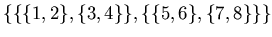(consider e.g., $v = 2$, $\tau = 3$, so the labels are structured in a tree as follows: $\{\{\{1,2\},\{3,4\}\},\{\{5,6\},\{7,8\}\}\}$) Consequently, a flat labeling with implicit ordering information is just as expressive as full hierarchical cluster trees. But let us return to labelings without ordering information.

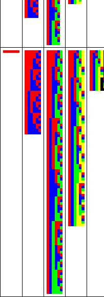
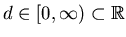
Figure 1.1: All possible clusterings of up to $n=6$ objects (rows top to bottom) into up to $k=6$ groups (columns left to right). In each table cell a matrix shows all clusterings for a particular choice of $n$ and $k$. A matrix shows one clustering per row. The color in the $j$-th column indicates the group membership of the $j$-th object. Group association is shown in red, blue, green, black, and gray.

Figure 1.1 illustrates all clusterings for less than 6 objects and clusters. For example, there are 90 partitionings of 6 objects into 3 groups. In general, for a flat clustering of $n$ objects into $k$ partitions there are

$$\frac{1}{k!} \sum_{\ell=1}^{k} \left( \begin{array}{c} k \ \ell \end{array} \right) (-1)^{k-\ell} \ell^n$$ (1.1)

possible partitionings, or approximately $k^n / k!$ for $n \gg k$. Clearly, the exponentially growing search space makes an exhaustive, global search prohibitive. In general, clustering problems have difficult, non-convex, objective functions modeling the similarity within clusters and the dissimilarity between clusters. In general, the clustering problem is NP-hard [HJ97].

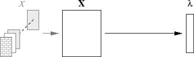
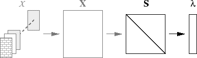
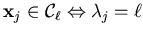
Figure 1.2: Object-centered (top) versus relationship-based clustering (bottom). The focus in this dissertation is on relationship-based clustering which is independent of the feature space.

In this dissertation, the focus is on the similarity space. Most standard algorithms spend little attention on the similarity space. Rather, similarity computations are directly integrated into the clustering algorithms which proceeds straight from feature space to the output space. The introduction of an independent modular similarity space has many advantages, as it allows us to address many of the challenges discussed in the next section. We call this approach similarity-based or relationship-based or graph-based. Figure 1.2 contrasts the object-centered with the relationship-based approach. The key difference between relationship-based clustering and regular clustering is the focus on the similarity space $\mathcal{S}$ instead of working directly in the feature domain $\mathcal{F}$.

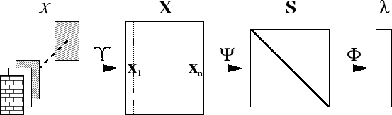
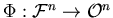
Figure 1.3: Abstract overview of the general relationship-based, single-layer, single-learner, batch clustering process from a set of raw object descriptions $\mathcal{X}$ to the vector of cluster labels $\mathbf{\lambda}$: $(\mathcal{X} \in \mathcal{I}^{n}) \stackrel{\Upsilon}{\rightarrow} (\mathbf{X}... ...\rightarrow} (\mathbf{\lambda} \in \mathcal{O}^{n} = \{ 1 , \ldots , k \}^{n})$

In figure 1.3 an abstract overview of the general relationship-based framework is shown. In web-page clustering, for example, $\mathcal{X}$ is a collection of $n$ web-pages. Extracting features yields $\mathbf{X}$, for example, the term frequencies of stemmed words, normalized such that $\forall \mathbf{x} \: \Vert \mathbf{x} \Vert _2 = 1$. Similarities are computed, using e.g., cosine based similarity $\Psi$ yielding the $n \times n$ similarity matrix $\mathbf{S}$. Finally, $\lambda$ is computed using e.g., graph partitioning.